Data Search - Weeks 7&8 Lab/Midterm
In weeks 7-8 we combined concepts learned up to this point to create maps with many key features including: Cities & towns, major waters, public lands,
As expected, this lab/midterm was the most challenging and time consuming yet, but I realized how much I have learned since day one - a lot. The most challenging part of this lab to me was finding an appropriate vector layer for each field and overcoming lag and errors within the ArcGIS software. Previously, the directions have been pretty straight forward, but when allowed a lot of room for creativity, I recognized that ArcGIS is not very accommodating to trial and error.
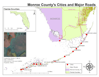
The main concern I had about this lab was that clipping the DEM and roads to the layer of Monroe County caused it to look splotchy and unfinished. I felt this took away from the purpose of the maps, so I left the other counties in and did the best job I could to make Monroe County stand out. I decided to include my process summary again this week because it explains my experiences with each map:
Process Summary
1.
First, I downloaded an aerial raster for the Flamingo
area in Monroe County. I chose Flamingo because it was the only city in the
FL_Cities layer on the main peninsula of Florida. I referred to the Week 6 lab
to make sure I downloaded the file correctly.
2.
Then, I downloaded each of my desired vector,
environmental, and raster layers from LABINS and FGDL. This process included a
lot of trial and error because the description of the layers in my search
results were often vague and I needed to insert the layers onto my map to see
how they actually looked and if they were appropriate.
3.
The first map I worked on was my CitiesRoads map
which includes Cities and Major roads of Monroe County. I realized while
working on this layer that the oddly shaped archipelago of the Florida Keys made
it difficult to clip any of my layers to the shape of the county, so I was forced
to leave the surrounding counties visible, but did my best to highlight and
differentiate Monroe County on the map. This meant that I couldn’t isolate the
roads in Monroe County because the main road through the keys would disappear over
water when clipped to the shape. Also, the mainland of Monroe County only had
one major road since it is mostly the everglades. For these reasons, I left the
roads visible on the neighboring counties. My aerial image is included on this
map.
4.
The next part I worked on was my
InvasivesLandCover map. I included these two datasets in one map because I felt
that it would be good to compare the amount of vegetation on the land to the
density of the invasive, exotic plants. In the view of the entire county, the
specific invasive points are not distinguishable, but the map still
communicates how many invasives there are. I decided to leave the aerial
picture so that the invasives were actually distinguishable in the area near
Flamingo. I used clip to shape on this map because it provided additional
clarity and to demonstrate I know how to do it since it affected the legibility
of the DEM in the next map.
5.
The final map I completed was my StateParksWater
map. As noted previously, the shape of Monroe County made the map messy when I
clipped the DEM to the shape of Monroe County, so I chose not to do that for
this map. Again I left the aerial photo in this map to provide more detailed
view of that area and to establish uniformity through the three maps.


Comments
Post a Comment